Threshold Models

Definition

Threshold Models denote a class of non-linear Credit Risk models where the credit standing (Credit Rating State) of an obligor is modelled in relation to the realization of a Random Variable (or stochastic process) versus predefined threshold values (also Barrier Models). This random variable (sometimes denoted Distance to Default) aims to capture and represent Creditworthiness. Threshold Models have affinity with Structural Credit Models of Default but need not be defined in terms of option theoretic assumptions.

Model Variations

There is a large variety of possible credit threshold models. Some key dimensions are indicatively:

• The Role of thresholds in model construction. For a large class of models, thresholds are inputs and the threshold crossing probabilities (transition rates) are outputs. In the complementary (inverse) problem, transition rates are the inputs and the threshold levels are produced as outputs
• The underlying stochastic process. Any category of stochastic process can be used in conjunction with a threshold crossing problem. Some interesting variations are:
  • The nature of the marginal distributions of the stochastic process (e.g. whether they are Gaussian or a more intricate distributions)
  • The autoregressive / mean reverting features of the stochastic process
• The use of continuous versus discrete time: Tractable (analytically solvable) threshold problems are typically defined in continuous time

The Canonical Model

The canonical (most studied and used) threshold model is built around Gaussian processes (or Brownian motion in the continuous time case). The underlying process is $X_k$ and evolves over different time periods according to

$X_k = X_{k-1} + \xi_k$

where $\xi_k$ are independent random variables distributed normally with zero mean and unit variance

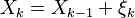
Credit Migration Thresholds

Given a Transition Matrix and the corresponding set of conditional threshold crossing probabilities $T^{mn}_{k}$ per rating class the task is to obtain a set of thresholds $A^{mn}_{k}$ that are consistent with these values.

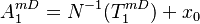
The Default Thresholds

The default thresholds $A^{mD}_k$ are special because they are absorbing. Default events are signaled by the first exit times of $X_k$ from suitable levels $A^{mD}_{k}$. The calculation of $A^{mD}_{k}$ beyond the first period requires the forward evolution of conditional (on non-default) probability density of the process $X_k$. We construct this survival density of the process iteratively

The Migration Thresholds

The thresholds are defined implicitly via the equalities

$\begin{array}{lllll} T^{mD}_{k} & = & P( \bigcup\limits_{l=1}^{k} (X_l < A^{m D}_l)) & & \\ T^{mn}_{k} & = & P( (A^{mn}_k < X_k < A^{m \,n-1}_k) \bigcap\limits_{l=1}^{k-1} (X_l > A^{m D}_l) ) & : & m<n \\ T^{mm}_{k} & = & P( (A^{m\,m+1}_k < X_k < A^{m\,m-1}_k) \bigcap\limits_{l=1}^{k-1} (X_l > A^{m D}_l) ) & & \\ T^{mn}_{k} & = & P( (A^{m\,n+1}_k < X_k < A^{mn}_k) \bigcap\limits_{l=1}^{k-1} (X_l > A^{m D}_l) ) & : & m>n \\ T^{m1}_{k} & = & P( (X_k > A^{m1}_k) \bigcap\limits_{l=1}^{k-1} (X_l > A^{m D}_l)) \end{array}$

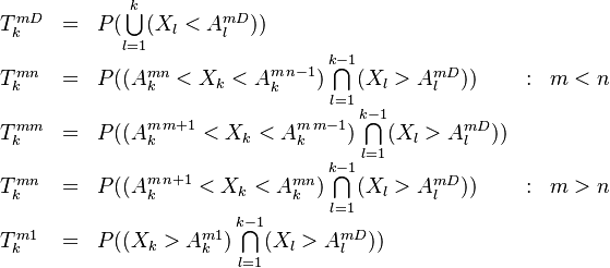
For each initial rating m, this is a system of $k \times D$ equations for the same number of unknowns. For a "default-only" approach, a recursive algorithm for obtaining the thresholds has been presented in .

Single Period Algorithm

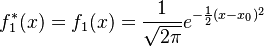
The first period density of the process is given simply by

$f_{1}^{*}(x) = f_{1}(x) = \frac{1}{\sqrt{2\pi}} e^{-\frac{1}{2}(x - x_0)^2}$

The first period threshold consistent with a crossing probability of $T^{mD}_1$ must satisfy the condition

$T^{mD}_1 + \int^{\infty}_{A^{mD}_1} dx f_{1}^{*}(x) = 1$

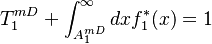
which expresses the fact that in the first period the process either lands beyond the threshold or not. This equation must be inverted to obtain $A^{mD}_1$ (we simplify here the notation by dropping the $mD$ indexes) For the first period the threshold is obtained via

$A^{mD}_1 = N^{-1}(T^{mD}_1) + x_{0}$

Multiperiod Algorithm

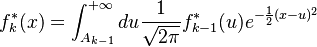
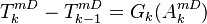
Once we have bootstrapped the first period density and threshold, subsequent periods are obtained by the Chapman-Kolmogorov equation. The survival density at step k is given by the convolution of the survival density at the previous step with the transition density:

$f_{k}^{*}(x) = \int^{+\infty}_{A_{k-1}} du \frac{1}{\sqrt{2\pi }} f_{k-1}^{*}(u) e^{-\frac{1}{2}(x - u)^2}$

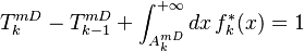
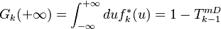
The default threshold $A^{mD}_k$ for each period k is given by the normalization condition

$T^{mD}_{k} - T^{mD}_{k-1} + \int^{+\infty}_{A^{mD}_{k}} dx \, f_{k}^{*}(x) = 1$

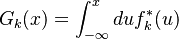
If we denote $G_{k}(x)$ as the distribution of the survival density up to point k:

$G_{k}(x) = \int^{x}_{-\infty} du f_{k}^{*}(u)$

Then equation becomes

$T^{mD}_{k} - T^{mD}_{k-1} = G_{k}(A^{mD}_{k})$

The distribution satisfies

$G_{k}(+\infty) = \int^{+\infty}_{-\infty} du f_{k}^{*}(u) = 1 - T^{mD}_{k-1}$

Recursive Solution

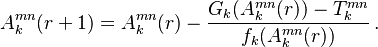
An efficient approach is based on Newton-Raphson: Let $A_k(r)$ denote the r-th iterated estimate of the threshold $A_k$. The recursion reads:

$\begin{array}{lll} A_{k}(r+1) & = & A_{k}(r) - \frac{G_{k}(A_{k}(r)) - p_{k}}{f^{*}_{k}(A_{k}(r))} \\ f^{*}_{k}(A_{k}(r)) & = & \int^{+\infty}_{A_{k-1}} du \frac{1}{\sqrt{2\pi}} f^{*}_{k-1}(u) e^{-\frac{1}{2}(A_{k}(r)- u)^2} \\ G_{k}(A_{k}(r)) & = & \int^{A_{k}(r)}_{-\infty} dx \int^{+\infty}_{A_{k-1}} du \frac{1}{\sqrt{2\pi}} f^{*}_{k-1}(u) e^{-\frac{1}{2}(x- u)^2} \\ & = & \int^{+\infty}_{A_{k-1}} du f^{*}_{k-1}(u) \int^{A_{k}(r)}_{-\infty} dx \frac{1}{\sqrt{2\pi}} e^{-\frac{1}{2}(x- u)^2} \\ & = & \int^{+\infty}_{A_{k-1}} du f^{*}_{k-1}(u) N(A_{k}(r) - u) \end{array}$

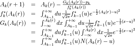
To obtain migration thresholds we replace in the equations above the period-k default probability $p_k$ with the appropriate transition probability $T^{mn}_k$.

$A^{mn}_{k}(r+1) = A^{mn}_{k}(r) - \frac{G_{k}(A^{mn}_{k}(r)) - T^{mn}_{k}}{f_{k}(A^{mn}_{k}(r))} \, .$

---