Equity Correlation Matrix

Definition

A Equity Correlation Matrix denotes a measure (or a model) of dependency between different corporate entities that is inferred from the co-movement of the their equity values. An equity correlation matrix is a special case of a Correlation Matrix and thus inherits properties and shares in the limitations and issues of that more general class.

Usage

• As a tool in the analysis of investment portfolios (usually as component of a larger set of data and model assumptions)
• As an input to measures of the likelihood of Joint Default in the context of Credit Portfolio Management, which in turn are used for Concentration Risk measurement

Construction

The construction of an equity correlation matrix involves an number of steps and assumptions:

• The selection of data sources
• The identification of precise data content and transformation of data to the desired form
• The selection of a modelling framework:
  • A minimal framework focusing on the empirical estimation of correlation via a number of possible dependency estimates
  • A factor model framework that aims to reduce the complexity of the correlation matrix by reducing the number of estimated parameters
  • A hierarchical, cluster or network dependency framework that selectively restores some pairwise relationships

Data Sources

The data sources for estimating an equity correlation matrix are the historical prices of traded instruments (shares). Relevant considerations (selection options) when constructing a sufficient data sample for the estimation of an equity correlation matrix are:

• The nature of the equity instruments traded (common stock, preferred stock etc.)
• The nature of the market(s) where the instruments are traded (trading platform, liquidity etc.)
• The precise data collected as determined by choices as:
  • The observation time (e.g closing)
  • Type (e.g. mid-market)
• The frequency of the sampling (e.g weekly)
• The length of the time window

Some issues that are relevant but elaborated on elsewhere:

• Stock Market Data may be subject to significant Data Quality issues.
• Corporate events (such as stock splits) may require special treatment (adjusted share price) to preserve the economic meaning of the data

Data Content and Transformations

Once the optionality in the selection of data sources discussed in the previous section is addressed the data set comprises of

• A number of distinct Timeseries Data $S^k_i$ where k denotes an observation timepoint and i is an index running over the entities in the sample
• Optionally, the classification of corporate stock using external information (e.g., business sector, country of operation etc.) using a set of index functions $I(i), C(i)$ etc that map individual entities to additional categories. In the simplest case these classifications or mappings are one-to-one (i.e., one entity to a single sector or region), but economically there may be multiple sectors, regions etc. that are applicable
• It is further possible to integrate the above data sets with further timeseries, e.g. economic / macro variables to enable a richer set of possible dependency models. Such more general models are not in scope of this article

The market data will typically be the levels (actual prices) of the traded instruments. Equity correlation matrices are estimated based on the log-returns of levels

$r^k_{i} = \log(S^{k+1}_{i}) - \log(S^k_{i})$

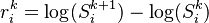
Sample (Empirical) Correlation Matrix

The pairwise sample correlation between two entities is derived by the standard Pearson correlation coefficient

$\rho_{ij} = \frac{\sum\limits_{k=1}^n (r^k_i - \bar{r_i}) (r^k_j - \bar{r_j})} {\sqrt{\sum\limits_{k=1}^n (r^k_i - \bar{r_i})^2 \sum\limits_{k=1}^n (r^k_j - \bar{r_j})^2}},$

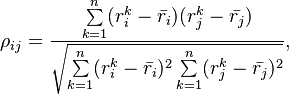
Alternative correlation measures (Spearman, Kendall) as listed in Correlation Matrix are advisable when assessing dependency but are more difficult to work with in a modelling context.

Correlation Matrix Models

In applications one typically requires constructing the joint distribution of returns $\mathbf{R}$ based on the historical data (and possibly additional classification information). The modelling process may involve a number of further (typically simplifying) assumptions. The result of adopting a model is that the model inferred correlation between any two entities is no longer the empirical correlation estimate but a model implied correlation

Some common model assumptions are:

• The means and variances of returns are not considered (These inputs may well be used in other portfolio management contexts)
• Correlations are stationary over time (More general classes of time-varying correlation models are available)
• Returns are distributed according to a given multivariate distribution function (copula) (Non-parametric, empirical copula approaches are also possible)
• Assumptions about the number and nature of the underlying model factors determining the correlation matrix

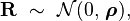
The Multivariate Normal Model

The conceptually simplest "model" is the direct use of the sample correlation matrix as the covariance matrix of a multivariate normal distribution. This model has the advantage that is using "all the information" in the data (up to linear level)

$\mathbf{R}\ \sim\ \mathcal{N}(0,\, \boldsymbol\rho),$

This approach is straightforward and suitable for concrete applications but it has some limitations:

• When the size of the equity universe is large the correlation matrix is unwieldy to understand
• When an entity's equity is not actively traded it might be difficult to include

General Multi-Factor Models

Multi-factor models aim to simplify the correlation matrix by imposing some structure and reducing the number of estimated parameters. The general form is:

$r^k_{i} = b_1 F^k_1 + \ldots + b_m F^k_m + e^k_i$

A more general version reads:

$r^k_{i} = b^i_1 F^k_1 + \ldots + b^i_m F^k_m + e^k_i$

• The m random variables $F_s$ are denoted common factors
• The m coefficients $b_s$ are denoted factor loadings
• The random variables $e^k_i$ are denoted idiosyncratic returns, error terms or residuals
• The distribution of all variables is assumed Gaussian

In the above expressions the factor loadings and/or the common factors are to be estimated statistically.

The factor realizations, $F^k_m$, are stationary with the following unconditional moments

$\begin{align} E[F_m] & = 0 \\ cov[F_m] & = E[F_m^2] = \Omega_f \end{align}$

The error terms are uncorrelated across time and entities and with the factors

$\begin{align} cov[e_j, e_i] & = 0 \\ cov[F_m, e_i] & = 0 \end{align}$

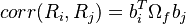
The equity correlation matrix produced by the model is given by:

$corr(R_i, R_j) = b_i^T \Omega_f b_j$

Latent Multi-Factor Models

Latent multi-factor models aim to simplify the correlation matrix on the basis of its own statistical properties (Sometimes called statistical factor models). In the simplest class of models, a linear multi-factor model assumes that the individual equity return is linked to a limited number of unobservable factors, with the relationship described by a linear equation.

This model is closely related to Principal Component Analysis which also summarises the structure of the correlation matrix

Fundamental Factor Models

Fundamental factor models are different from latent factor models. Here the observable asset characteristics like industry / country classifications are used to construct simplified representations that are useful in portfolio management context.

There are two distinct types of fundamental factor models:

• The factors are known and one estimates the loadings
• The loadings are known and one estimates the factors

Models with Known Factors

These models are loosely inspired by the CAPM and APT asset pricing theories

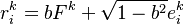
The Single-Factor Model

This is an important special case of the multi-factor model, interesting for its simplicity and underpinning conceptually the asymptotic single factor risk model of Basel II. It is sometimes denoted the Single-index model.

Depending on the generality of the loadings $\alpha$ we can distinguish three subcategories

Uniform Loadings

All equities are assumed to share the same loading to the single factor

$r^k_{i} = b F^k + \sqrt{1 - b^2} e^k_i$

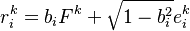
Grouped Loadings

Equities are grouped in subsets that share the same loading to the single factor

$r^k_{i} = b_{I(i)} F^k + \sqrt{1 - b^2_{I(i)}} e^k_i$

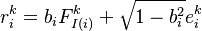
Individual Loadings

Equities are assumed to have individual loadings to the single factor

$r^k_{i} = b_{i} F^k + \sqrt{1 - b^2_{i}} e^k_i$

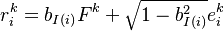
Credit Metrics like Models

This is a simplified multifactor model where the equity value of each entity is assumed to be linked to the industrial / regional sector it is classified to belong

$r^k_{i} = b_i F^k_{I(i)} + \sqrt{1 - b^2_i} e^k_i$

where $F^k_{I(i)}$ is the industry/regional index to which the entity i is mapped via the function $I(i)$

Moody's GCorr like Models

A more complex hierarchical factor model

Models with Known Loadings

Barra-like Models

In such models the loadings of individual returns to factors are given (e.g. industry classification).

$r^k_{i} = b^i_1 F^k_1 + \ldots + b^i_m F^k_m + e^k_i$

The system is solved to derive the factors $F^k_m$

More Complicated Models

Macroeconomic Factor Approaches

Other approaches to developing correlation matrices may involve use of additional data in the form e.g. of macroeconomic timeseries. In those models Macroeconomic Factors are added to the equity data as covariates (explanatory factors). These models are more complex as they involve timeseries of distinctly different nature

Copula Models

Relaxing the rather strict linearity and Gaussianity assumptions leads to the general class of copula models where they multivariate dependency can be governed by more complex functional forms

Issues and Challegnes

• It is sometimes easy to confuse the notions of a correlation matrix as an empirical estimate versus the the implied correlation that is the outcome of a multi-variate model
• The matrix derived from pairwise correlation estimates may fail to be positive semi-definite (exhibit negative eigenvalues). Such a matrix cannot be used directly for modelling purposes and must be converted into a valid Correlation Matrix first.
• In the context of credit applications measures of equity correlation is used sometimes as a proxy for the desired but more difficult to obtain Asset Correlation Matrix which involves additional assumptions and potential Model Risk

See Also

• Asset Correlation Matrix

---